
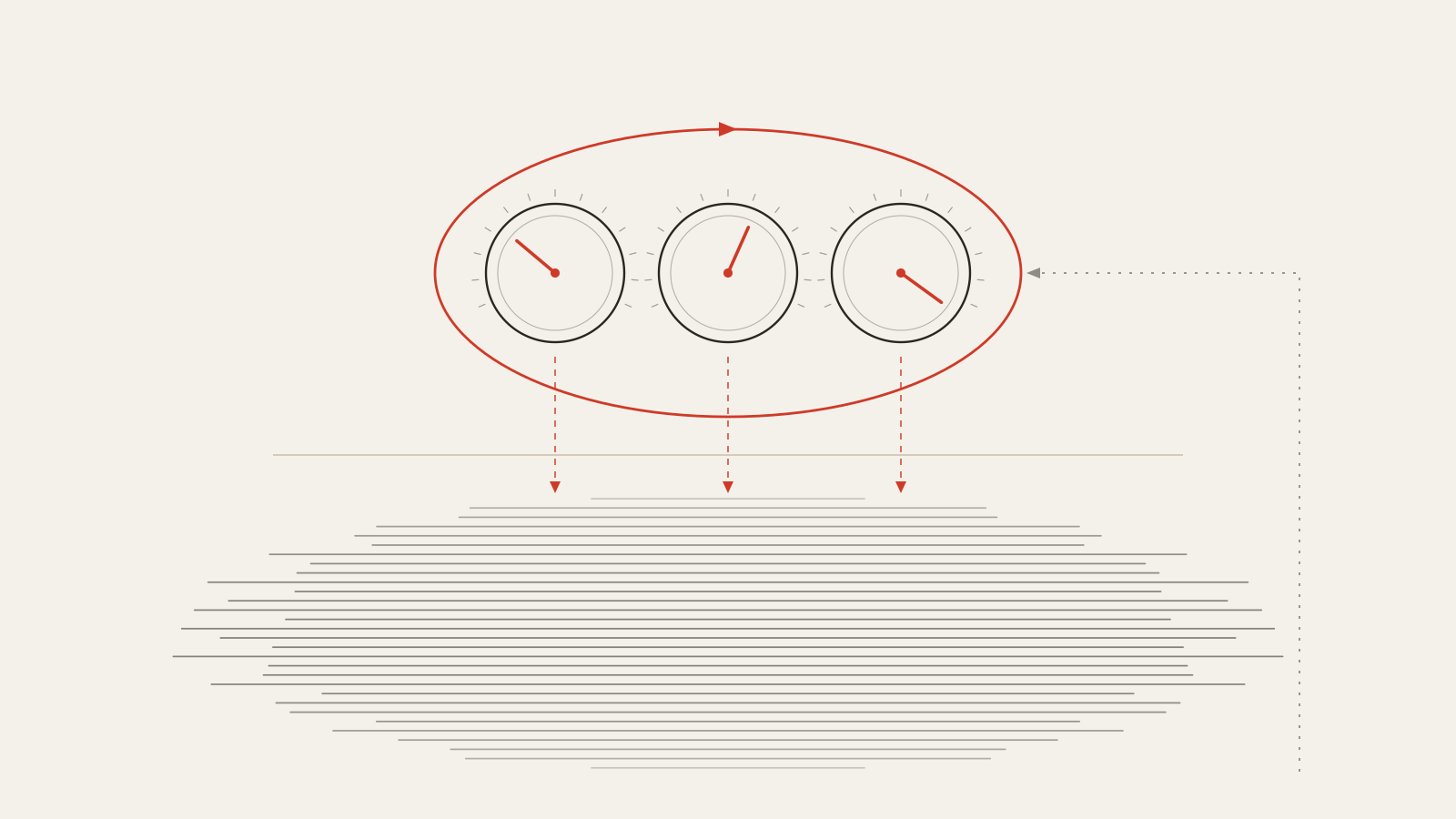
A Meta agent turns the dials of a production recommender every three days. It doesn’t rank items or retrain models: it touches the control surface, around ten calls per cycle, and the estimated cost of the whole loop stays in the tens of dollars. An appendix to the loops series.
This series has climbed one step per instalment. First came the loop: sensor, controller, effector, measurement, round again — homeostasis with a GPU, emptying a backlog while you sleep. Then the graph, once it became clear that the agent forgets and the graph doesn’t. And in the third, the graph stopped being a drawing and became the program: nodes that think, edges that are code, judgment × topology.
All three had something in common that I never said out loud: the loop lived inside my computer. The backlog was mine, the repo was mine, and if the creature made a mess, it made it on a branch.
This appendix is about what happens when that same pattern leaves the IDE and gets plugged into a system serving billions of people. On 2 September, ten authors at Meta AI put a short, remarkably unpretentious paper on arXiv called CORAL — Constraint-Optimized Recommender via an Agentic Loop — accepted at the OARS workshop at RecSys ’26. It is, as far as I know, the first decent public description of an agentic loop running on a production recommender, with real A/B experiments and measured numbers.
And the interesting part isn’t the numbers. It’s where they chose to plug the model in.
Two planes, and almost everyone picks the wrong one
When someone says “let’s put an LLM in the recommender,” the default mental image is one of two things: the model ranking the items, or the model understanding the user in order to rank the items better. Either way, the LLM ends up in the data plane: on the path every request travels, between the user and what they see.
That plane has one property that ruins everything: cost scales with traffic. One call per request, or per item, or per user. Multiply that by a billion-user surface and you’re no longer doing engineering, you’re doing a spreadsheet that doesn’t balance. Add latency: the model is now on the critical path of something that has to answer in milliseconds.
CORAL does the opposite. The model observes the system only through aggregate signals. And what it touches are the controls.
A large recommender, the authors note, “is not a single model but a large, multi-stage system — candidate retrieval, ranking, and serving.” That system is full of knobs: how much retrieval budget each candidate source gets, which serving treatment each user segment receives, how much aggressiveness, how much caching, how much prefetching. The paper calls that set the control surface, and each knob a control unit. One line from the paper — written about the retrieval sources’ budget shares — explains both why this matters and why nobody looks at it: those shares “are typically hand-set and seldom revised.”
That’s where the agent lives. In the control plane. It doesn’t decide what a user sees: it decides how the system that decides what a user sees is configured.
The economic consequence is severe enough to be worth reading slowly, and I work through the formula below. But the headline is this: in the control plane, the number of model calls doesn’t depend on traffic. It depends on how many decision groups you carved your control surface into. A handful per cycle. The same whether you have a thousand users or a billion.
The anatomy, piece by piece
If you read the first instalment, the skeleton will look familiar to the point of discomfort. It’s exactly the same loop, with different names and a different budget.
What it observes. Aggregate operating statistics per control unit, plus recent changes. No individual events.
What it remembers. Here’s the first piece worth stealing. Memory isn’t a drawer: it’s three stores with distinct jobs.
- The observation store holds the raw per-unit statistics.
- The assessment store holds “concise, natural-language judgments of which parts of the system are performing well or poorly and how their behavior is trending.”
- The decision store holds the configurations the agent previously deployed together with the outcomes later attributed to them.
That third one is what makes this an actual loop rather than a well-written proposal generator. An agent that remembers what it did but not what happened next isn’t learning: it’s drafting. The memory horizon is m = 3 cycles.
What it acts with. A small set of deterministic tools — five, counting the one that deploys — and the division of labour is the third instalment’s thesis taken to its limit — save the agents for judgment, plumbing is code:
| Tool | What it does | Who’s in charge |
|---|---|---|
| Analysis | Computes and summarizes statistics from raw observations | Code |
| Retrieval | Surfaces the relevant history from memory | Code |
| Attribution | Estimates the effect of the previous configuration | Code |
| Constrained optimizer | Projects the proposal onto the budget-feasible set | Code |
| Deployment | Applies the accepted configuration to the live recommender | Code |
The model doesn’t compute. The model reads what the tools computed, reasons over it, proposes a bounded adjustment and writes down why. That rationale isn’t decoration: it’s what lets a human supervise, and what feeds the next cycle’s attribution.
How often. k = 3 days per cycle. And I like that they’re honest about where the number comes from: “long enough for a configuration’s effect to surface in the metrics, yet short enough for the agent to act promptly on what it observes.” Followed by the sentence half the field would have quietly omitted: “We chose these as sensible defaults rather than tuning them.”
What closes the loop. An A/B experiment. Not a test going green: a production experiment spanning millions of users whose result is written to the decision store and becomes the next cycle’s context.
The model proposes, arithmetic disposes
This is the piece I’m taking with me into every loop I build from now on, and it’s simple enough to be annoying.
The agent doesn’t deploy what it proposes. It proposes bounded per-unit adjustments, and that proposal goes through an optimizer that returns “the closest configuration that satisfies the operating budget — the projection of the proposal onto the budget-feasible set {s : c_t(s) ≤ B}.”
Read that again with operations eyes. The budget constraint isn’t asked of the model. It isn’t in the prompt as a polite “please don’t overspend.” It doesn’t depend on the model having understood the arithmetic correctly on a Tuesday afternoon. It’s in the structure: whatever the model proposes comes out of the optimizer feasible by construction.
That’s the difference between a guardrail and a suggestion. And it’s the real reason, I think, that this can ship to production without anyone’s hands shaking: the worst case of a hallucinating model isn’t a seven-figure invoice, it’s a bad proposal that the projection turns into a mediocre feasible configuration, that the A/B measures as neutral, and that the next cycle corrects.
The authors put it less dramatically: the split means “the model contributes judgment while the tools supply computation and hard guarantees.”
The reward function is an A/B test
The first case study is a video-recommendation service. The control units are the retrieval sources — the different mechanisms that contribute candidates — and a configuration assigns each one a budget multiplier within a bounded range. The operating cost is the total retrieval budget consumed.
Three rounds, measured with A/B:
- Round 1, a zero-shot proposal formed from a single window of statistics: +0.13% watch time, sessions neutral.
- Round 2: the agent shifted budget more aggressively between sources, overcorrected, and the measured effect was neutral.
- Round 3, which aggregates several decision cycles and is the deployed configuration: +0.15% watch time, +0.16% sessions across all users, and +0.77% sessions in the largest market. All of it at no additional serving cost, because the reallocation consolidated the retrieval budget rather than expanding it.
And here’s the detail almost everyone would read as a failure. The paper flags it itself, correctly: “this progression is not monotonic — the second round did not improve on the first — yet it is precisely the behavior the loop is designed to produce.”
Think about it from the first instalment. A loop that only goes up isn’t a loop: it’s a streak. What proves there’s real feedback is exactly this — the agent overshot, the A/B told it so, it read that in its own decision store, and the next round corrected. The measured error is the signal.
They then extended the setup to produce distinct allocations per segment — engagement level and account tenure — and that’s where the number I find most telling appears: +0.23% sessions for new low-signal users. The agent shifted budget toward the sources that lean on content and context signals, the ones that hold up when you know almost nothing about the user, and away from those that depend on history. It’s a call any reasonable engineer would have made. The point is that nobody made it, because that knob was hand-set and almost never revised.
The other screw: serving capacity
The second case is a different service and a different class of decision, with the same loop. Here the control units are user segments, and each is assigned a serving treatment from a discrete menu: variants in retrieval aggressiveness, ranking, caching and prefetching. The constraint is a fixed serving-cost cap.
- Round 1: working within a subset of user segments, the agent reduced serving cost substantially, “saving millions of USD in annualized capacity expenditure.”
- Round 2: reading that result against its previous decision, the agent recognized the same change could safely be applied to more segments, widened the allocation and increased the first round’s savings by 44%, while leaving engagement “statistically unchanged.”
Careful with that 44%, the number most likely to be retold wrong: it is not a 44% saving. It’s 44% more saving than the previous round. If round one saved X, round two saved X·1.44.
That the same harness works for pushing engagement in one place and cutting cost in another is the paper’s generality argument, and it’s a fair one: the authors present it as evidence that “a single agentic loop can take on continual optimization work traditionally performed by human algorithm engineers, with a path from human-supervised operation toward autonomous operation under guardrails.”
The bill: why this costs tens of dollars
Here’s the thesis of the whole piece, and it’s purely architectural.
The cost of the entire setup is:
Cost = (T / k) · C · (τ_in · p_in + τ_out · p_out)where T is the deployment length in days, k the cadence in days, C the number of model calls per cycle, τ the average input and output tokens per call, and p the per-token prices.
Three properties fall out, and the third is the one that matters:
- Cost is inversely proportional to cadence. Shorter cycles = more responsiveness at proportionally higher cost. You get an explicit dial between the two.
- It’s bounded per cycle, since
τ_outcan’t exceed the model’s output-token limit. No long tail. - And the good one:
C“is fixed by how the control surface is partitioned into decision groups (a handful per cycle), not by the number of users or requests served, so the cost is independent of traffic and remains negligible even on billion-user surfaces.”
The figures they give for the two deployments are almost comically small — and it’s worth stressing that they are estimates “from prompt and payload sizes,” because, as the table caption itself admits, “the pipelines do not log token usage”:
| Deployment | Calls/cycle | Input tokens/call | Output tokens/call |
|---|---|---|---|
| Retrieval budget | ~10 | ~1,500 | ~2,500 |
| Serving capacity | ~8 | ~2,000 | ~2,500 |
Each cycle issues a handful of calls of a few thousand tokens each, so a deployment of several cycles totals “on the order of 10⁶ tokens,” placing the end-to-end inference cost of each deployment “on the order of tens of U.S. dollars — negligible against the engagement gains and operating-cost savings it produces.”
One million tokens. Against millions of annualized dollars saved in the second case. That asymmetry isn’t the model’s magic: it’s the geometry of where you plugged it in.
And the sentence that captures the change in the job, verbatim from the paper: “compressing a tuning cycle from several engineer-weeks to a few autonomous days, an order-of-magnitude faster turnaround with no engineer in the loop.”
The small print
This is the section I care about most, and the reason I like this paper despite everything missing from it. It’s short, it’s a workshop paper, and it should be read for what it demonstrates rather than what it suggests.
| What’s easy to read into it | What the paper says when you trace it |
|---|---|
| “Gains of 0.13% to 0.77%, statistically solid” | There is not a single confidence interval, p-value or exact N in the entire paper. All there is is a binary label in the Table 1 caption: “neutral denotes no statistically significant change.” You can infer the rest are significant, but it’s never asserted cell by cell and no uncertainty magnitude is given. |
| “The LLM beats the human engineer” | There is no competitive baseline. Not against an engineer, not against bandits, not against Bayesian optimization, not against RL. Only A/B against the production control. What’s demonstrated is that the loop improves on a configuration hand-set and seldom revised — which is exactly what the authors claim. |
| “A frontier model achieved…” | The paper never names the model. Not the family, not the vendor. It says “a general-purpose language model,” and “frontier-LLM” appears only as a pricing reference for the cost estimate. The tens-of-dollars figure is an estimate with representative pricing, not an invoice — and the Table 2 caption admits the tokens weren’t measured either: “the pipelines do not log token usage.” |
| “Three rounds, three decisions” | Round 3 “aggregates several decision cycles and is the deployed configuration.” It isn’t one turn: it’s several. |
| “It runs on its own” | “Although the loop runs autonomously, it still operates under human supervision.” Strengthening the automated guardrails so that supervision “can be reduced” is declared a natural next step. |
| “It works for any lever” | “Both studies instantiate the harness on a single class of decision — the constrained allocation of a recommender’s resources across its components.” Extending it to retrieval and ranking logic itself is listed as pending. |
And one limitation the authors themselves flag as an open problem, which I find the most honest of the lot: the evidence comes from A/B experiments, which measure real effects but are “costly to run and specific to their setting.” There is still no standardized way to evaluate agent-driven system optimization before deploying it. Which means: to find out whether your loop works, for now you have to let it loose in production.
Also: no code, no project page, no data. Nothing reproducible. And a final curiosity, for those of us who watch these things: the paper is filed on arXiv under cs.CL, computation and language. Not cs.IR, not cs.LG. A recommender-systems paper in the computational linguistics category says a fair amount about which field this team thinks it’s working in.
What I’m taking back to my own loop
Scale aside, which isn’t replicable, there are five design decisions here that are, and that I’m adopting:
- Separate the plane. Before putting a model into anything, ask whether it goes on the path of every request or on the path of the configuration. If it’s the configuration, cost stops scaling with usage and latency stops mattering. There’s almost always a version of your problem that lives in the control plane.
- Make constraints structural, not textual. Any limit you ask of the model in the prompt is a suggestion. Any limit you impose by projecting its output onto a feasible set is a guarantee. If your agent has a budget, a quota or a cap, put it in a function, not in a paragraph.
- Store decisions with outcomes, not just observations. The store that makes the loop learn is the one pairing “what I deployed” with “what happened next.” Without that pair you have an agent with a diary, not a memory.
- Pick cadence from your signal’s latency.
kisn’t tuned by searching for an optimum: it’s chosen by how long an effect takes to become visible. And since cost is inversely proportional tok, that number is simultaneously your responsiveness dial and your spending dial. - Expect the bad round. If your loop improves on every turn, suspect the measuring device. The round that overshoots and gets corrected is the proof that feedback exists.
Verdict
The pattern yes, the extrapolation no. What CORAL demonstrates is narrow and solid: an agent in a closed loop, with memory of its own consequences and constraints baked into the structure, can sustain the continual tuning of a production system better than a configuration hand-set and seldom revised, at a cost that disappears into rounding. What it doesn’t demonstrate — and doesn’t claim to — is that an LLM is the best tool for that job: the missing baseline is the one comparing it against the classical constrained-optimization methods that have been doing exactly this for decades.
But the architectural lesson holds entirely, and it closes this series better than I closed it myself. The first instalment left a formula: your leverage is skill × clarity. The third added a factor: judgment × topology. This appendix adds the last one, and it’s the one that decides whether the loop can leave your laptop:
surface × cadence. Which dials your loop can touch, and how often it can measure what happened when it touched them.
Everything else — the model, the prompt, the memory, the tools — is implementation. If the control surface is small, the loop can’t change anything that matters. If the cadence is faster than the signal, the loop learns noise. And if nobody is measuring the outcome in production, then you don’t have a loop: you have an agent writing very convincing proposals that nobody has ever checked.
The creature left the IDE. Turns out there are dials out here.
Ideas over code; evidence over hype.
References
- Azhar, M. R., Zhou, Y., Jiang, G., Wang, Y., Sharma, R., DeSousa, M., Liu, J., Guo, X., Zhang, L. & Fan, X. (2026). CORAL: An LLM-Native Harness for Production Recommender Systems. arXiv:2609.02730 [cs.CL], 2 September 2026. Accepted at the RecSys ’26 OARS Workshop.
- Earlier instalments in the series: The creature that empties your backlog while you sleep, The agent forgets, the graph doesn’t and The creature no longer waits in line: dynamic workflows and the jump from chain to graph.

Leave a Reply